Note
Click here to download the full example code
Use ASE to Simulate Planetary Motion
This tutorial shows how to use ASE to simulate planetary motion. Although both ASE and NNP are designed for molecular dynamics (MD), implementing a force field to do MD is not at a reasonable abount of work to use as a tutorial. So we simulate something different here. Assume we have two atoms, one hydrogen and one carbon. They are all moving under the gravity centered at the origin. There is no interaction between these two atoms.
Let’s first import all the packages we will use:
import ase
from ase.data import atomic_masses
from ase.units import fs
from ase.md.verlet import VelocityVerlet
import nnp.md as md
import pytest
import sys
import math
import matplotlib.pyplot as plt
The module nnp.md provide tools to run molecular dynamics with a potential defined by PyTorch. To define the potential we need to provide a function that takes the chemical symbols, atom coordinates, unit cell, and PBC flag as an input and returns the molecular energy as an output. The output and input coordinates and cell must be in the a differentiable graph so that PyTorch could automatically compute the force and stress tensor using the autograd engine. In this example, we don’t care about the periodic boundary condition and unit cell because we are actually not simulating molecular system.
From basic physics, we know that the equation for gravitational potential has the equation \(E(r)=-\frac{GMm}{r}\). For simplicity, we choose \(GM=1\) when \(E\) is in \(\mathrm{eV}\), \(m\) in \(\mathrm{amu}\), and \(r\) in Angstrom.
def gravity(chemical_symbols, coordinates, _cell, _pbc):
    assert len(chemical_symbols) == coordinates.shape[0]
    atomic_numbers = {'H': 0, 'C': 6}
    mass = coordinates.new_tensor(
        [atomic_masses[atomic_numbers[s]] for s in chemical_symbols])
    inv_r = 1 / coordinates.norm(dim=1)
    potential_energies = - mass * inv_r
    return potential_energies.sum()
with this potential, we could define an ASE calculator:
calculator = md.Calculator(gravity)
Now let’s create two atoms, initially at (1, 0, 0) and (2, 0, 0)
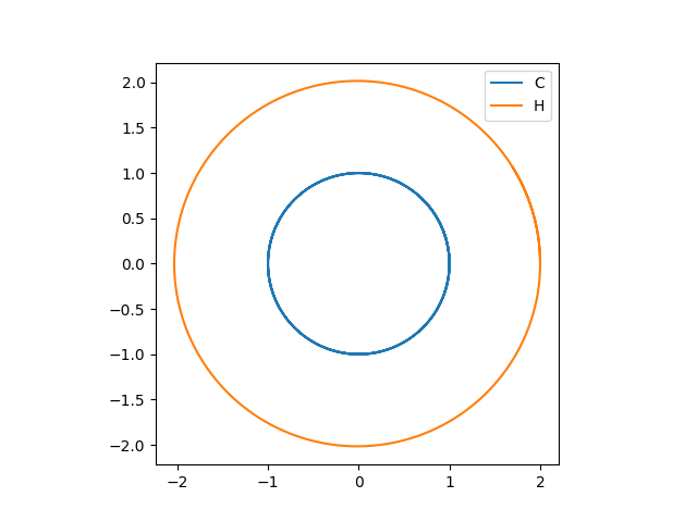
For the purpose of demonstration, we make these two atoms’s trajector a perfect circle at the XY plane. To do so, we need to carefully set the initial velocity. It is not hard to get that, the velocity is \(v = \sqrt{\frac{GM}{r}}\).
planets.set_velocities([[0, 1, 0], [0, 1 / math.sqrt(2), 0]])
planets.set_calculator(calculator)
Now we can start the dynamics:
Out:
True
Now let’s plot the trajectory to see what we get:

Out:
/home/runner/work/nnp/nnp/tests/planetary_motion.py:100: MatplotlibDeprecationWarning: Adding an axes using the same arguments as a previous axes currently reuses the earlier instance.  In a future version, a new instance will always be created and returned.  Meanwhile, this warning can be suppressed, and the future behavior ensured, by passing a unique label to each axes instance.
  plt.axes().set_aspect('equal')
To check the correctness of this dynamics, we use pytest to test if it is on the XY plane and if the trajectory is circle:
Out:
============================= test session starts ==============================
platform linux -- Python 3.7.7, pytest-5.4.3, py-1.8.2, pluggy-0.13.1 -- /opt/hostedtoolcache/Python/3.7.7/x64/bin/python
cachedir: .pytest_cache
rootdir: /home/runner/work/nnp/nnp, inifile: setup.cfg
collecting ... collected 2 items

planetary_motion.py::test_is_on_xy_plan PASSED                           [ 50%]
planetary_motion.py::test_is_circle PASSED                               [100%]

============================== 2 passed in 24.56s ==============================
Total running time of the script: ( 0 minutes 49.812 seconds)